Basics of Data Analysis for Storytelling

At a Glance

• Revisiting the Narrative
• What are our Analysis Questions?
• Walkthrough of Analysis
• How Did the Analysis Impact our Narrative?

Revisiting the Narrative

This is the third lesson in our series on Data Storytelling for Sports. In our last lesson, we covered exploring data to discover a narrative. In this lesson, we'll pick up where we left off and do a deeper set of analyses on the data. At this stage, we're going to explore things more deeply to see if our narrative holds or if we discover something new.

The question we started with was when do NHL superstars peak? And our goal in the last lesson was to explore the data to see what sort of narrative would emerge from this question. Now that we've completed our initial data exploration, our draft narrative is as follows:

• Two superstars stand above the rest, Wayne Gretzky and Mario Lemieux. They had different styles that were both effective and they were revered players that significantly impacted the era in which they played.

From our initial data exploration, a few things came to light, which are as follows:

• Wayne Gretzky and Mario Lemieux are significantly better than their superstar cohort using average Points per Game (PPG) by season.
• They had peaks at 23, but they also had multiple peaks in their career.
• They both played in an era where the league expanded and the game changed quite a bit.
• Both their styles of play contributed to the evolving of the sport.
• And both carried strong brands of their own.

Our goal now is to push on the above; to see if we can look at the data in a more methodical and analytical way. In real-world projects, this might mean an exploratory analysis followed by a more detailed analysis (e.g., correlation analysis, regression model, etc.) to answer specific questions. In this lesson, we'll keep the analysis relatively simple to illustrate how we can go about answering our specific questions.

Feeling lazy? Don't want to read? Check out our video accompaniment to this newsletter below.

What are our Analysis Questions?

We will divide our analysis into two phases: quantitative and qualitative. The quantitative phase will focus on statistical analyses and modeling. The qualitative phase is about background and research on the main character or actor in the data story.

Quantitative Questions

Three questions will guide our quantitative analysis:

1. At what age did each superstar peak?
2. Were there any superstars with multiple peaks?
3. How did the superstars compare to one another?

This should give us a profile of the superstar cohort and give us a relative sense for how Gretzky and Lemieux compared to that cohort. It should also help us discover some other interesting facts that may evolve our narrative.

Qualitative Questions

Two questions will guide our qualitative analysis:

1. What is the background for those superstars on whom we chose to focus?
2. Is there something unique or interesting about that superstar?

These quantitative and qualitative questions are obviously not exhaustive. So, be sure to spend some quiet time with a pen and paper and write down as many potential questions as possible. Then read through them to see which ones could draw out the best story and use those to guide your analysis.

Walkthrough of Analysis

For this email course, we've created a public GitHub repository for the data, analyses and code that you can use for the hands-on portions of the lessons.

For this lesson, you can find the data, code and analysis files in the Lesson 3 folder.

Note that we've included 108 years worth of player stats data in the Data folder. We used this file along with a list of the superstars we wanted to analyze to create a filtered dataset.

Review of Code Snippets

If you open the R code in the Data_Analysis folder, you'll see a file called age_of_decline_analysis.rmd. In this file, there are several code snippets. Let's briefly walk through each of them.

This first one loads the libraries we'll use in our analysis.

library(tidyverse)
library(zoo)

The second loads the 108 years worth of player stats.

nhl_player_stats_df <- read.csv("../Data/all_player_stats_1917_to_2024.csv")

The third creates a list of superstars that we used to filter the original dataset. If you want to change the list, you can edit the names in this list to expand or contract the players you want to analyze.

superstar_array = c("Wayne Gretzky", "Jaromir Jagr", "Mark Messier", 
                    "Gordie Howe", "Ron Francis", "Marcel Dionne",
                    "Steve Yzerman", "Mario Lemieux", "Sidney Crosby",
                    "Joe Sakic", "Alex Ovechkin", "Phil Esposito",
                    "Ray Bourque", "Joe Thornton", "Mark Recchi",
                    "Paul Coffey", "Stan Mikita", "Teemu Selanne",
                    "Bryan Trottier", "Adam Oates")
                    

This next code snippet filters the original dataset, calculates three new columns (GPG, APG and PPG) and creates a new data frame that is grouped by player name (and saves it as a CSV file).

filtered_data <- nhl_player_stats_df %>%
  filter(PLAYER_NAME %in% superstar_array)
  
superstar_df <- filtered_data %>% 
  select(SEASON, PLAYER_NAME, AGE, TEAM, POS, GP, G, A, PTS) %>% 
  mutate(
    GPG = round(G/GP, 3),
    APG = round(A/GP, 3),
    PPG = round(PTS/GP, 3)
  ) %>% 
  arrange(desc(PPG))
  
peak_ppg_season <- superstar_df %>%
  group_by(PLAYER_NAME) %>%
  filter(PPG == max(PPG, na.rm = TRUE)) %>%
  select(PLAYER_NAME, SEASON, AGE, PPG) %>%
  arrange(desc(PPG))

write.csv(peak_ppg_season, "peak_ppg_by_age.csv", row.names = FALSE)

This next code snippet creates a rolling average across three years and then calculates the peak PPG for that rolling average. It also saves the resulting data frame as a CSV file.

rolling_avg_data <- superstar_df %>%
  arrange(PLAYER_NAME, SEASON) %>%  
  group_by(PLAYER_NAME) %>%
  mutate(ROLL_3YR_PPG = rollmean(PPG, k = 3, fill = NA, align = "right")) %>%
  ungroup()

peak_rolling_ppg <- rolling_avg_data %>%
  group_by(PLAYER_NAME) %>%
  filter(ROLL_3YR_PPG == max(ROLL_3YR_PPG, na.rm = TRUE)) %>%
  select(PLAYER_NAME, SEASON, ROLL_3YR_PPG) 

write.csv(peak_rolling_ppg, "peak_3_yr_rolling_view.csv", row.names = FALSE)

This next code snippet then creates a data frame for multiple peaks (using a 90% threshold value). So, it includes other peak averages that are within 10% of the peak. Again, we save the data frame as a CSV for offline use.

superstar_df <- superstar_df %>%
  group_by(PLAYER_NAME) %>%
  mutate(PEAK_PPG = max(PPG, na.rm = TRUE),
         PEAK_THRESHOLD = 0.90 * PEAK_PPG,  
         IN_PEAK = PPG >= PEAK_THRESHOLD)   

peak_periods <- superstar_df %>%
  filter(IN_PEAK == TRUE) %>%
  select(PLAYER_NAME, SEASON, PPG)

write.csv(peak_periods, "multiple_peaks.csv", row.names = FALSE)

Multiple CSV files are now generated from the above code snippets, so you can analyze them in Microsoft Excel or your favorite analytical tool.

At What Age did Each Superstar Peak?

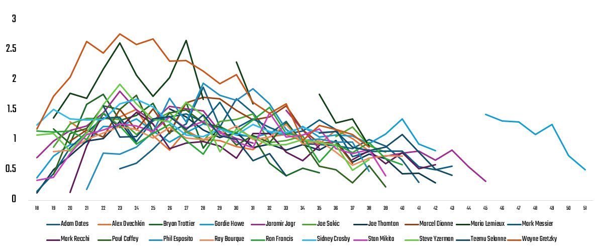
We looked at this in a couple of ways (both included in the aforementioned spreadsheet). The first was using a heatmap and the second through a trend view where we lay the data across each player's Age along the X-axis and then plotted the Points per Game by season on the Y-axis. This results in a multi-line graph; however, discerning (even visually) individual performance peaks is not easy. You get a general and cluttered sense of trending at best.

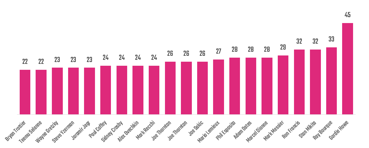
A simpler view was to take the R code that calculated age and peak performance and then plot this using a column chart. The below is the result. Note that some players had multiple peaks, so this takes the highest Points per Game value and the age when the player achieved it. This is a nice, simple view, but it doesn't lead us to understanding the average number of years it takes a superstar to peak, and the flow into and out of a peak year.

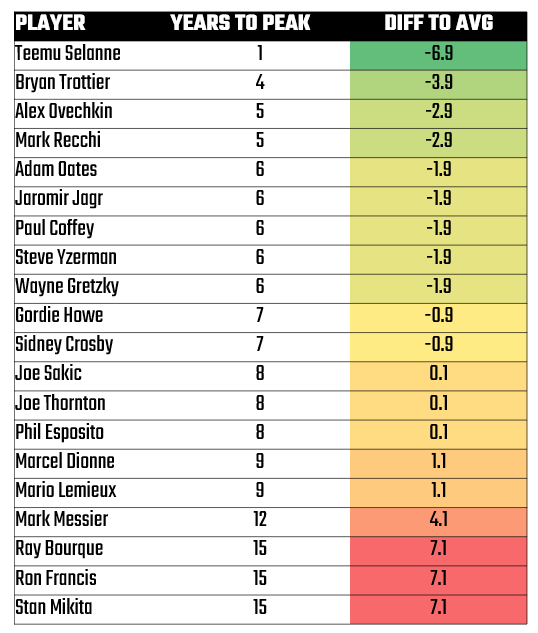
The below view begins to get at a more secondary level of information. That is, out of all of the superstars, the average number of years to get to peak performance is 7.9 years. This view shows a) the individual player's time to performance peak (YEARS TO PEAK) and b) the delta between their timeframe and the average (DIFF TO AVG).

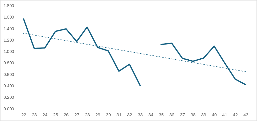
You can begin to see how additional analyses, even simple ones, can begin to tease out different stories. For example, We hadn't considered a story on Teemu Selanne, an amazing Finnish hockey player. He started strong, peaking in his first year of play, but subsequently declined (using PPG as the metric). That said, he still managed to have an amazingly long and productive career. Below is a view of his Points per Game (PPG) by season versus Age.

Were There any Superstars with Multiple Peaks?

The short answer is yes. For example, in the R code we showed earlier we created a data frame that surfaced the closest performance years to a superstar's peak year – within 10% of the peak year. Interestingly, we found 80% of the players had two or more peak years.

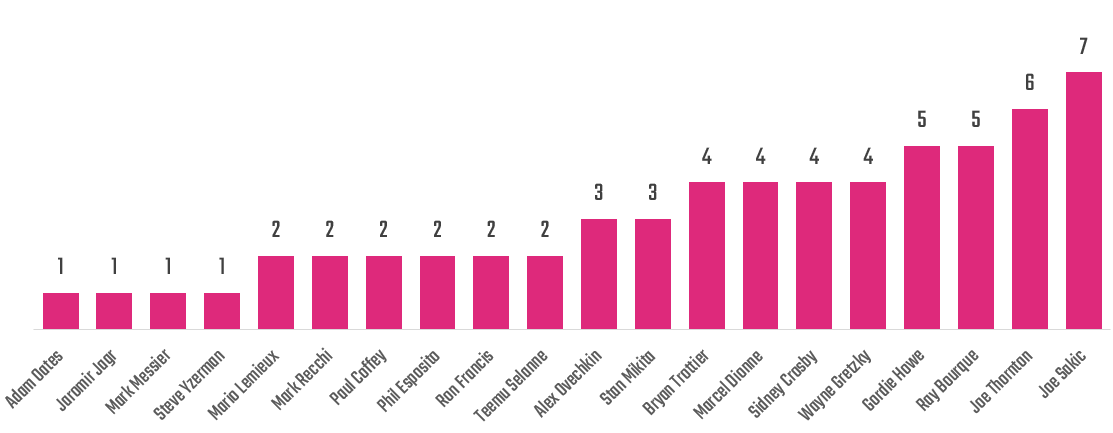
Again, another potential story that we had not anticipated emerged from this simple analysis: Joe Sakic's multiple peaks and consistency in play across his 20-year career or Jaromir Jagr's single peak in his twenty-year career.

How did the Superstars Compare to One Another?

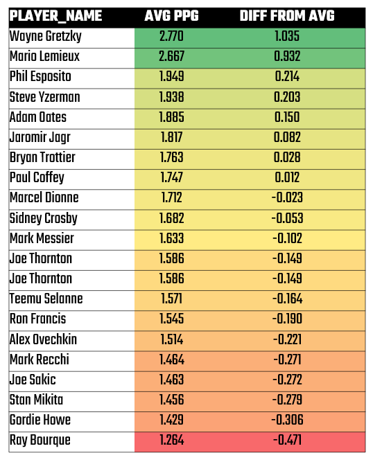
You can already see some of this based on the above analyses that we did. However, below we've summarized the Points per Game by season and then calculated the difference from the average. Now, if you stopped here, you might miss a lot of nuance, so it's important to think second-level on your analyses. For example, the positions of these players would impact their PPG as would the eras within which they played. That said, it's pretty clear that Wayne Gretzky and Mario Lemieux stand out. While a delta of ~1 may not seem like a huge number, it's significant: this delta represents approximately one more point per game that they were able to achieve when compared to their peers.

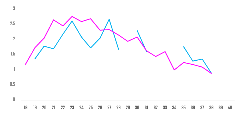
And if we stick on Gretzky (pink) and Lemieux (blue), you can see that Gretzky had a more natural arc to his career (even though he had multiple peaks earlier in his career) and Lemieux's career was more staccato and interrupted.

Now that we've spent some time on quantitative analyses, let's move to a more qualitative analysis of the narrative we're carrying forward.

What is the Background for those Superstars on Whom we Chose to Focus?

Wayne Gretzky and Mario Lemieux are two of the greatest players in hockey history, but they dominated in different ways. While Gretzky was the ultimate playmaker with unmatched consistency, Lemieux was a solid blend of size, skill, and scoring efficiency.

Gretzky’s dominance came from sustained excellence—he had 15 seasons with 100+ points and played 20 years without a significant drop-off. Lemieux, despite missing nearly 500 games due to injury and illness, had a similar Points per Game (PPG) rate at his peak.

Wayne Gretzky: "The Great One"

Wayne Gretzky, born on January 26, 1961, in Brantford, Ontario, is universally regarded as the greatest hockey player of all time. He dominated the NHL during his 20-season career, primarily with the Edmonton Oilers, but also with the Los Angeles Kings, St. Louis Blues, and New York Rangers.

Gretzky won four Stanley Cups with Edmonton (1984, 1985, 1987, 1988) and played a crucial role in expanding hockey’s popularity in the United States, especially in California after being traded to the L.A. Kings. He retired as the NHL’s all-time leader in goals, assists, and points, earning an immediate induction into the Hockey Hall of Fame in 1999.

Gretzky is the most dominant offensive player in hockey history and holds more NHL records (60+) than any other player, which include:

• Most career goals: 894
• Most career assists: 1,963
• Most career points: 2,857
• Most points in a single season: 215 (1985-86)
• Most 100+ point seasons: 15

Mario Lemieux: "Super Mario"

Mario Lemieux, born on October 5, 1965, in Montreal, Quebec, is one of the greatest hockey players of all time. Drafted first overall by the Pittsburgh Penguins in 1984, Lemieux transformed the franchise into a championship team. He played 17 seasons, all with Pittsburgh, winning two Stanley Cups as a player (1991, 1992) and three more as an owner (2009, 2016, 2017). He was inducted into the Hockey Hall of Fame in 1997, bypassing the usual waiting period due to his impact on the game.

Career-Defining Stats & Achievements

• 6x Art Ross Trophy winner
• 3x Hart Trophy winner
• 2x Conn Smythe Trophy winner
• 10th all-time in points (1,723) despite missing 500+ games
• 2nd all-time in points per game, behind only Wayne Gretzky

Lemieux was a generational talent whose career was cut short by injuries and illness, yet he still dominated every era he played in. His skill, perseverance, and legacy as both a player and an owner make him one of the most unique and impactful figures in hockey history.

Is there Something Unique or Interesting about that Superstar?

Wayne Gretzky

• His Hockey IQ Was Unmatched. Gretzky’s greatest asset wasn’t size or speed—it was his hockey sense and anticipation. He famously said, “I skate to where the puck is going to be, not where it has been.” His ability to read plays before they developed made him nearly unstoppable.
• The Office Behind the Net. Gretzky revolutionized offense by using the area behind the net as a playmaking hub, now referred to as “Gretzky’s Office.” From there, he set up countless goals, controlling the game with unparalleled vision.
• The Only 200-Point Player in NHL History. No other player has ever reached 200 points in a season. Gretzky did it four times (1981-82, 1983-84, 1984-85, 1985-86), peaking at 215 points in 1985-86.
• His Records May Never Be Broken. Many of Gretzky’s records are considered unbreakable, especially in the modern era of the NHL.

Mario Lemieux

• One of the Most Skilled Players Ever. Lemieux combined a rare blend of size (6’4”, 230 lbs), finesse, vision, and goal-scoring ability. He made the impossible look effortless, often weaving through defenders with smooth, long strides.
• Incredible Comeback Story. First, he overcame Hodgkin’s Lymphoma (1993). In one of the most legendary moments in NHL history, Lemieux received a radiation treatment for cancer in the morning, then flew to Philadelphia and scored a goal that same night. Despite missing 24 games, he won the 1992–93 Art Ross Trophy with 160 points in just 60 games. He retired in 1997 Due to Chronic Back Issues. He had suffered from herniated discs and sciatic nerve pain throughout his career. Then, he returned to the NHL in 2000 after 3½ years away and still dominated. His comeback season (2000-01) saw him score 76 points in 43 games at age 35.
• The Only Player to Own the Team He Played For. After retiring, Lemieux saved the financially troubled Pittsburgh Penguins from bankruptcy in 1999 by converting the team’s debt into equity. He became the first former player to own an NHL team, and under his ownership, the franchise thrived, securing new ownership stability, a new arena, and three more Stanley Cups.

How Did the Analysis Impact our Narrative?

Your data analysis should impact your narrative in some way. For example, you might discover that single stat that will be the main actor in your data story, or you may find events across a timeline that tell an interesting story. Either way, a good analysis helps bring your data story to life.

For our narrative, we noted several points that could be used within a data story. For example:

• Both Gretzky and Lemieux were anomalies when compared to their superstar peers. Gretzky achieved an average of 2.77 PPG and Lemieux 2.67 PPG.
• They also had strong supporting players around them, which helped them rise to high levels of stardom.
• Gretzky had a career with an uninterrupted arc that included multiple performance peaks. He also achieved 60+ records that may likely go unbroken.
• Lemieux had a great career, but suffered health issues that interrupted his career – twice. Imagine if he hadn't had those issues.
• Lemieux was also a player and an owner at the same time. This must have come with deep responsibility and pressure.

So, at this point you'll want to spend more time on your actual story.

In our next lesson, we'll spend more time on fleshing out the data story. As a primer, here are three examples of where you could end up.

• A timeline visualization that compares the statistics and events around Gretzky's and Lemieux's peaks.
• A What If Lemieux stayed healthy? model that projects a healthy Lemieux against Gretzky's actual stats.
• A modern NHL projection for both players to see how they would fare in a more modern hockey era.

We hope you followed along with the analysis, and if you did we would encourage you to write down potential stories of your own.

Summary

In this lesson, we conducted an analysis of the data to more closely examine the superstar cohort. We used questions to frame the analysis. We also broke the analysis into a quantitative phase and a qualitative phase. The quantitative phase helped us discover specific metrics and values, and the qualitative phase helped us discover more background information and unique traits that could help structure the story.

Now that we've explored some of the basics in data analysis, the next step is to start mapping out our data story. In the next lesson, we’ll take key data points, statistics and qualitative notes from this week's lesson and start to brainstorm what a potential data story might look like.

Subscribe to our newsletter to get the latest and greatest content on all things Data, AI and Design!